Getting started with ggsunburstR • ggsunburstR

Overview

ggsunburstR creates sunburst and icicle plots from hierarchical data using ggplot2. It accepts multiple input formats and produces standard ggplot2 objects you can customise freely.

Basic usage

The workflow has two steps:

Prepare data with sunburst_data()
Plot with sunburst(), icicle(), donut(), or ggtree()

library(ggsunburstR)

# Parse a Newick tree string
sb <- sunburst_data("((a, b, c), (d, e, f));")

# Sunburst plot
sunburst(sb, fill = "depth")

# Same data as an icicle plot
icicle(sb, fill = "depth")

Input formats

Newick strings

The most common input for phylogenetic or hierarchical trees:

sb <- sunburst_data("((mammals, birds, reptiles)vertebrates, (beetles, flies)insects)animals;")
sunburst(sb, fill = "name")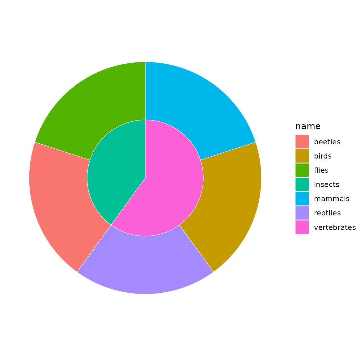

Data frames

Use a data frame with parent and child columns:

df <- data.frame(
  parent = c(NA, "root", "root", "fruits", "fruits", "vegs", "vegs"),
  child  = c("root", "fruits", "vegs", "apple", "banana", "carrot", "pea")
)
sb <- sunburst_data(df)
sunburst(sb, fill = "name")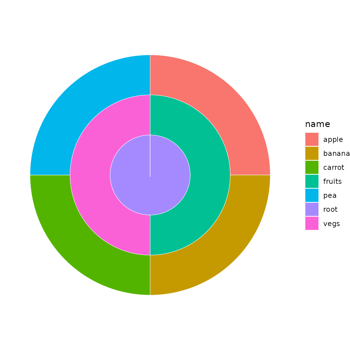

Path-delimited strings

Hierarchies can also be expressed as slash-delimited paths:

sb <- sunburst_data(c("A/B/C", "A/B/D", "A/E/F"))
sunburst(sb, fill = "name")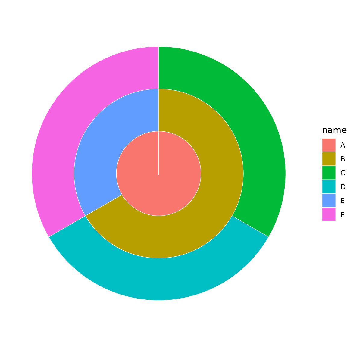

Other formats

ggsunburstR also accepts Newick files, node-parent CSVs, lineage TSVs, ape::phylo objects, and data.tree::Node objects. See ?sunburst_data for details.

Plot types

Donut charts

A donut is a sunburst restricted to the outermost depth levels:

sb <- sunburst_data("((a, b, c), (d, e, f));")
donut(sb, fill = "name", levels = 1, hole_size = 2)

Tree dendrograms

ggtree() renders the tree as a dendrogram:

sb <- sunburst_data("((a:0.3, b:0.5)X:0.2, (c:0.4, d:0.1)Y:0.3)root;")
ggtree(sb, show_labels = TRUE)

Value-weighted sectors

By default, all leaves get equal angular width. Use values to size sectors proportionally:

sb <- sunburst_data(
  "((a, b, c), (d, e));",
  values = c(a = 10, b = 5, c = 3, d = 8, e = 2)
)
sunburst(sb, fill = "name")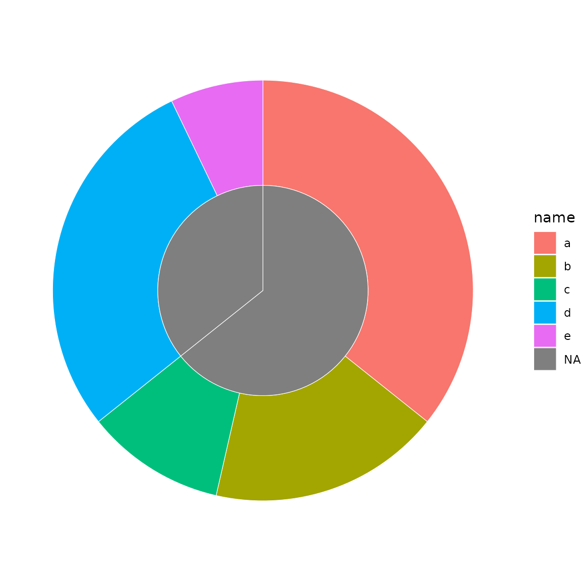

Fill mapping

The fill parameter accepts column names (quoted or bare), plus the special values "auto" (maps to depth) and "none" (static grey):

sb <- sunburst_data("((a, b, c), (d, e, f));")

# Bare name (tidy eval)
sunburst(sb, fill = depth)

# Auto-map to depth
sunburst(sb, fill = "auto")

Labels

Basic labels

Add leaf labels with show_labels = TRUE:

sb <- sunburst_data("((a, b, c), (d, e, f));")
sunburst(sb, fill = "depth", show_labels = TRUE)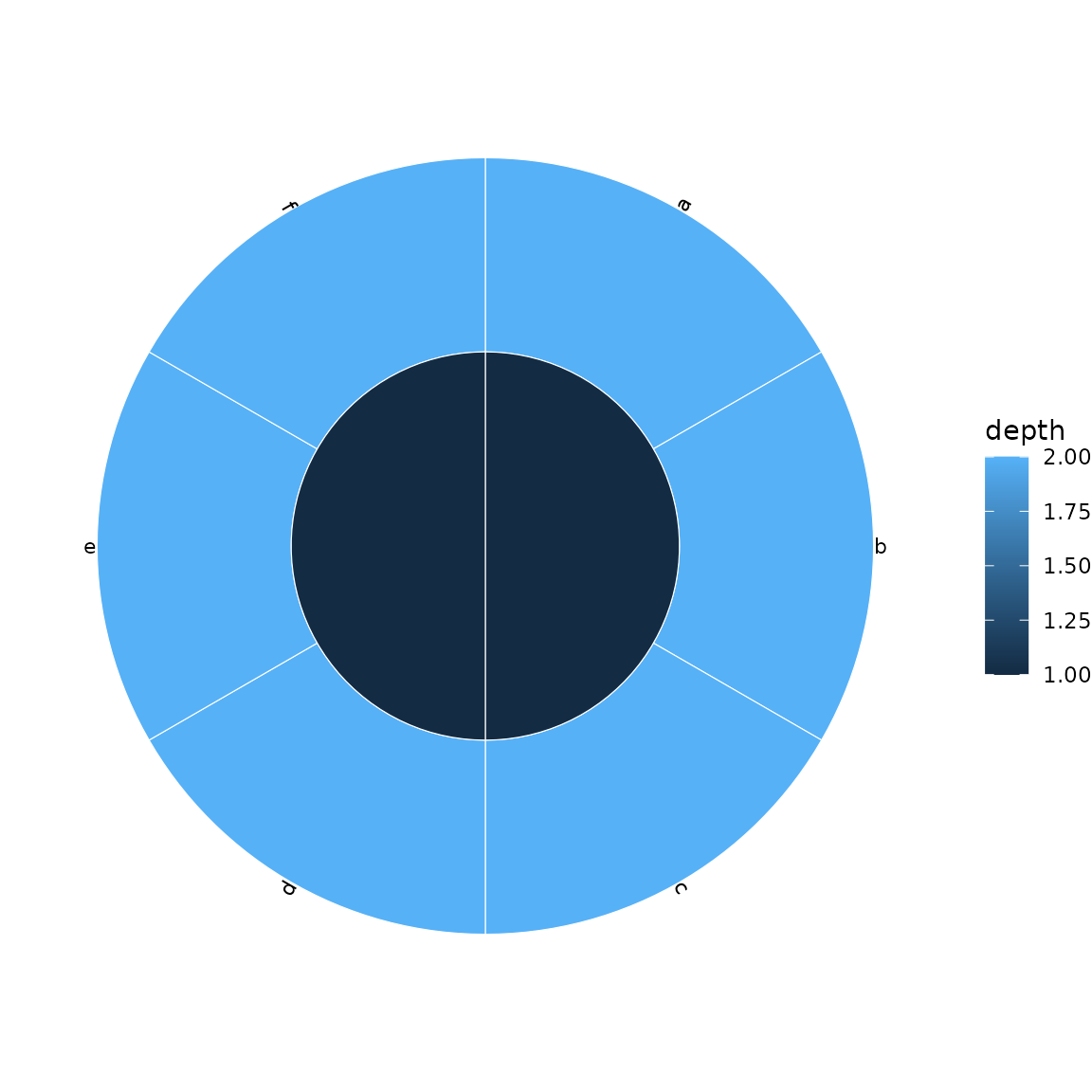

Perpendicular labels

Use label_type = "perpendicular" for arc-following labels:

sunburst(sb, fill = "depth", show_labels = TRUE,
         label_type = "perpendicular")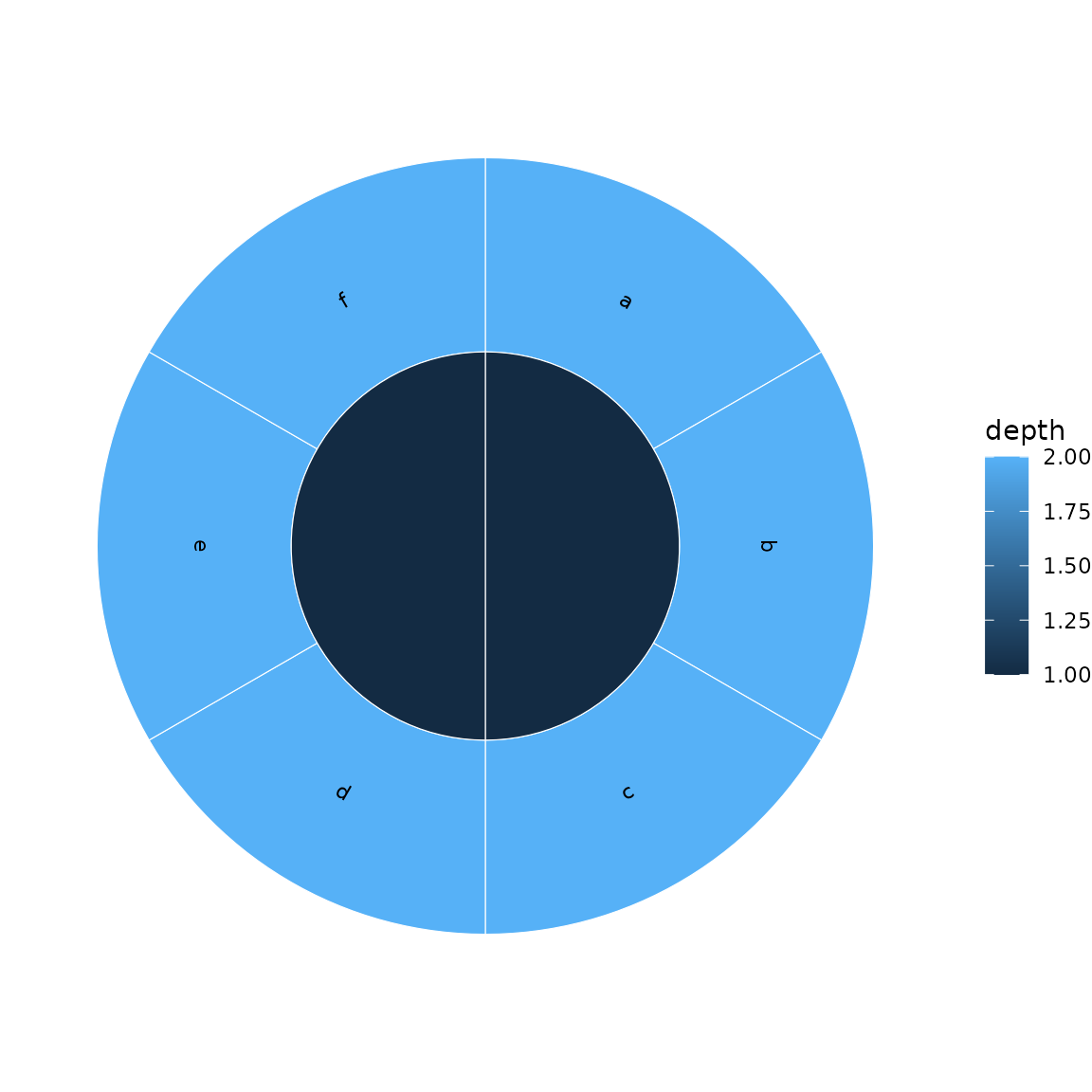

Internal node labels and filtering

Show labels for internal nodes and filter out labels on narrow sectors:

sb <- sunburst_data("((mammals, birds, reptiles)vertebrates, (beetles, flies)insects)animals;")
sunburst(sb, fill = "name", show_labels = TRUE,
         show_node_labels = TRUE, min_label_angle = 30,
         label_size = 3.5)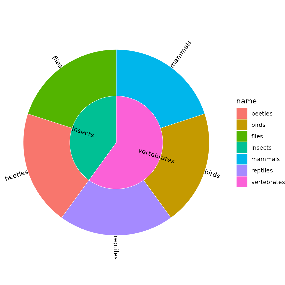

Label repulsion (icicle)

Use ggrepel for collision avoidance in icicle plots:

sb <- sunburst_data("((a, b, c, d, e), (f, g, h));")
icicle(sb, fill = "depth", show_labels = TRUE, label_repel = TRUE)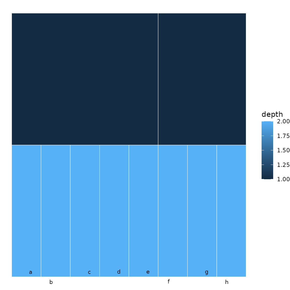

Drilldown into subtrees

Zoom into a specific branch with drilldown():

sb <- sunburst_data("((a, b)X, (c, d)Y)root;")
sub <- drilldown(sb, node = "X")
sunburst(sub, fill = "name")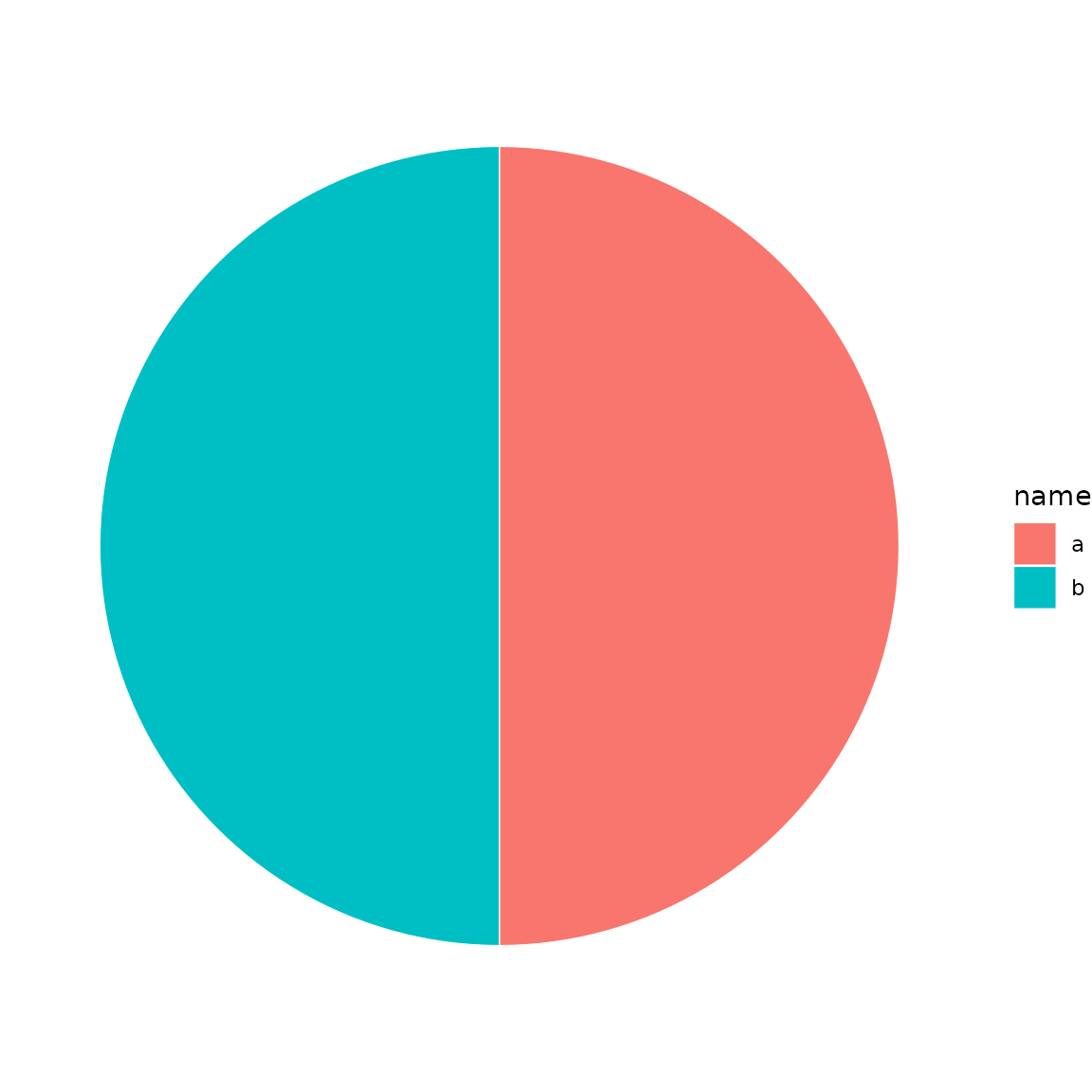

Annotations

Bar chart annotations

Add bar charts adjacent to leaf nodes:

df <- data.frame(
  parent = c(NA, "root", "root", "root"),
  child  = c("root", "A", "B", "C"),
  score  = c(NA, 0.5, 0.9, 0.3)
)
sb <- sunburst_data(df)
p <- icicle(sb, fill = "name")
bars(p, sb, variables = "score")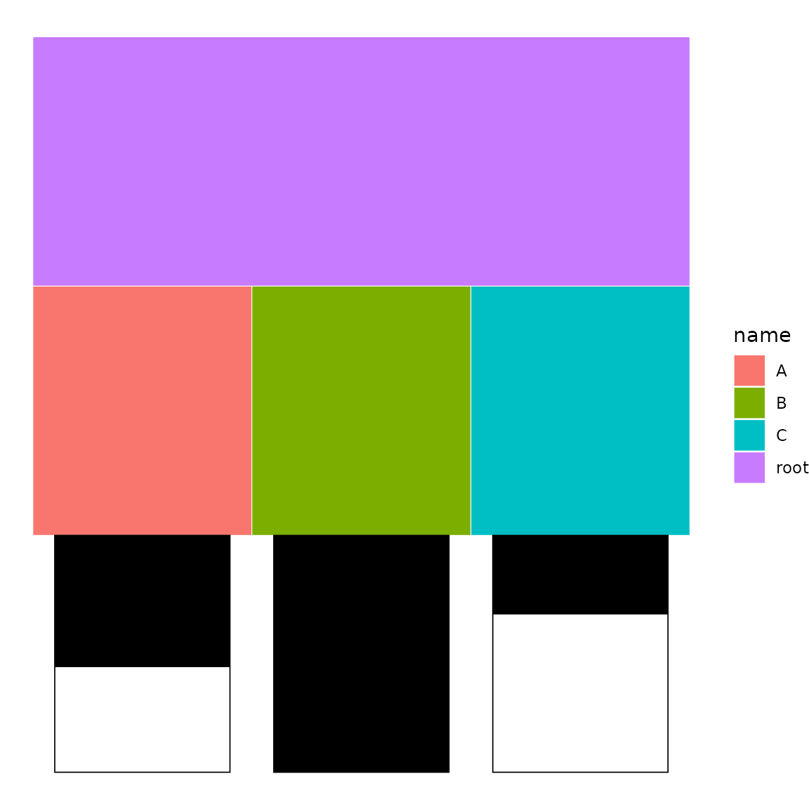

Tile (heatmap) annotations

Add colour-coded tiles adjacent to leaf nodes:

df <- data.frame(
  parent = c(NA, "root", "root", "root"),
  child  = c("root", "A", "B", "C"),
  group  = c(NA, "x", "y", "x")
)
sb <- sunburst_data(df)
p <- icicle(sb, fill = "name")
tile(p, sb, variables = "group")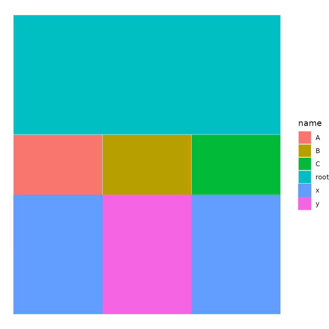

Highlight specific nodes

Emphasise nodes by name or ID:

sb <- sunburst_data("((a, b, c), (d, e));")
p <- sunburst(sb, fill = "depth")
highlight_nodes(p, nodes = c("a", "c"), fill = "red")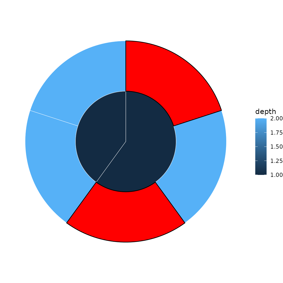

Per-depth fill scales

Use sunburst_multifill() or icicle_multifill() to map different colour scales to different hierarchy levels:

sb <- sunburst_data("((a, b)X, (c, d)Y)root;")
sunburst_multifill(sb, fills = list("1" = "name", "2" = "name"))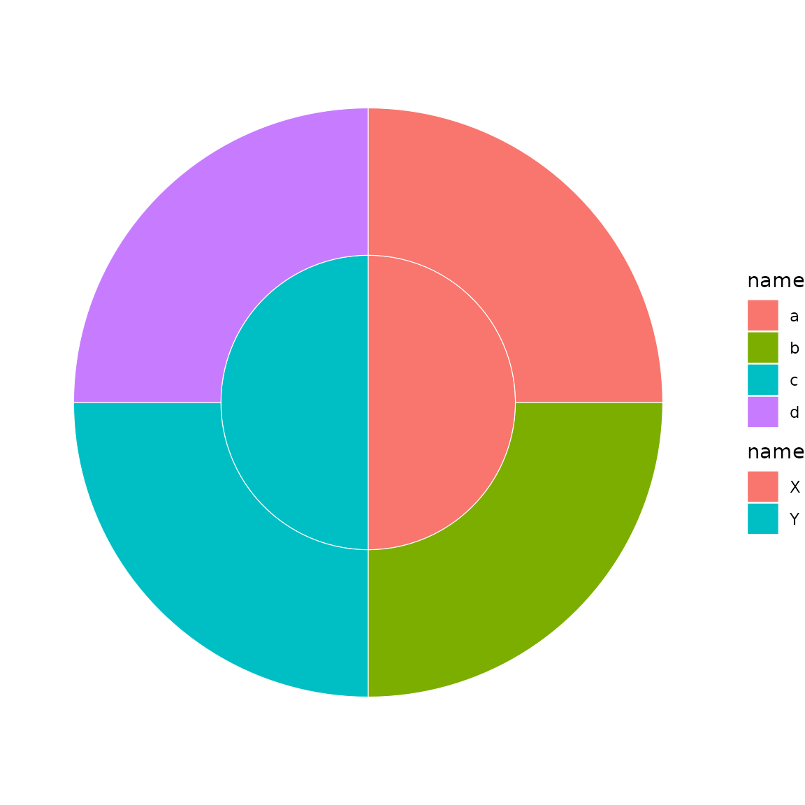

ggplot2 geom

For idiomatic ggplot2 syntax, use geom_sunburst() directly with a data.frame:

df <- data.frame(
  parent = c(NA, "root", "root", "A", "A"),
  child  = c("root", "A", "B", "a1", "a2"),
  group  = c("r", "g1", "g2", "g1", "g1")
)

ggplot2::ggplot(df) +
  geom_sunburst(ggplot2::aes(id = child, parent = parent, fill = group)) +
  ggplot2::coord_polar() +
  theme_sunburst()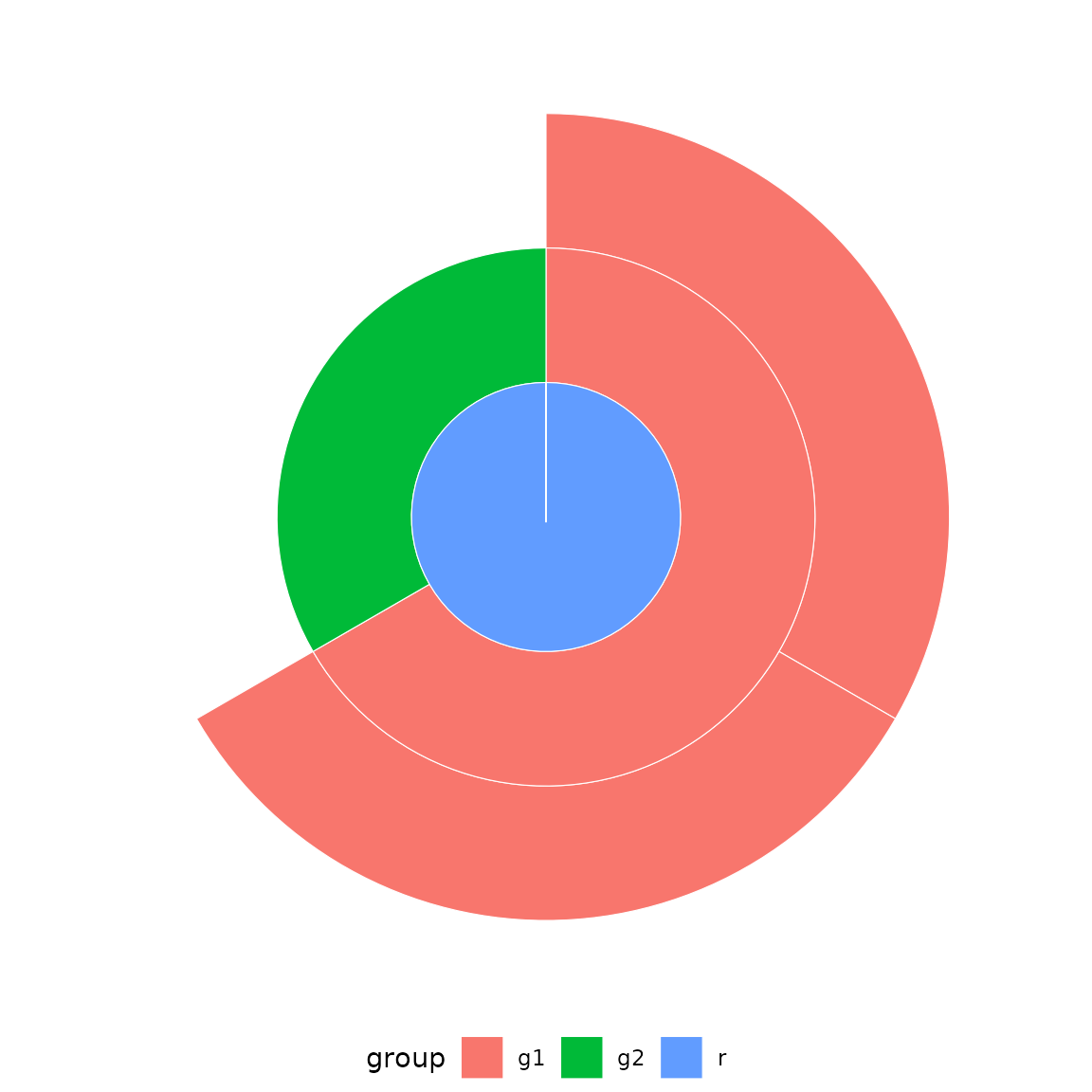

Tree inspection

Use nw_print() to inspect tree structure:

nw_print("((a, b)X, (c, d)Y)root;")
#> 
#> Phylogenetic tree with 4 tips and 3 internal nodes.
#> 
#> Tip labels:
#>   a, b, c, d
#> Node labels:
#>   root, X, Y
#> 
#> Rooted; no branch length.

Customisation with ggplot2

Since the output is a standard ggplot2 object, you can add any ggplot2 layer or theme:

sb <- sunburst_data("((a, b, c), (d, e, f));")
sunburst(sb, fill = "name") +
  ggplot2::scale_fill_brewer(palette = "Set2") +
  ggplot2::labs(title = "Custom sunburst") +
  theme_sunburst()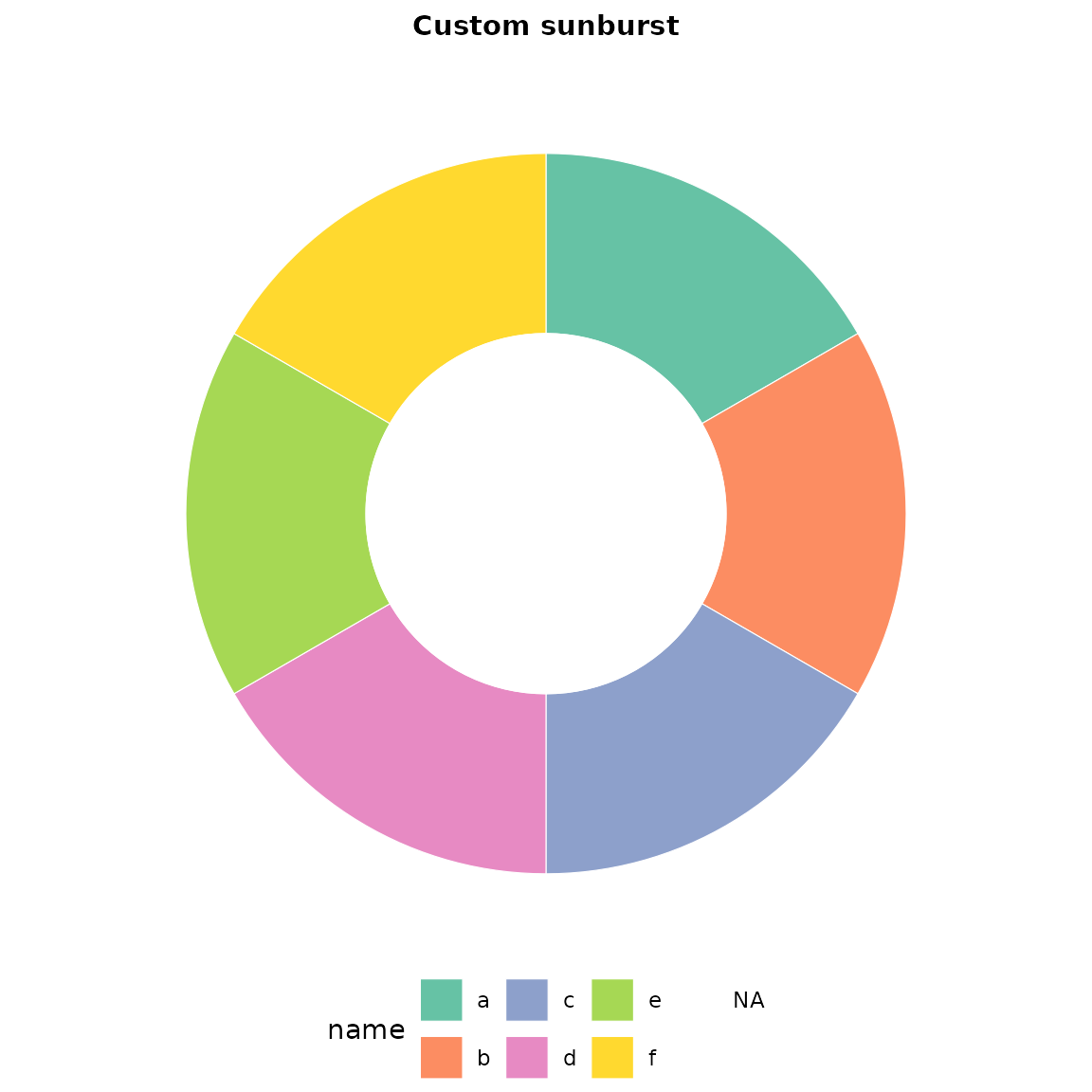

Options

Key parameters for sunburst_data():

values — named numeric vector or column name for sector sizing
branchvalues — "remainder" (default) or "total"
leaf_mode — "actual" (default) or "extended"
ladderize — sort by descendant count
ultrametric — equalise leaf depths
xlim — angular span (default 360)
rot — rotation offset in degrees